
Night 2:The Microquasar Wakes Up
More hours
More hours
With the significance we have, we can’t go very far. No one is going to take us seriously if we don’t get 5 sigmas.
We need more observation hours to see if with more statistics the significance rises (good!) or disappears (arghhh!). But even that will be difficult with less than 3 sigmas.
How easy it would it be to call Daniel who is operating the telescopes and tell him to keep pointing at Cyg-X1, right? But it’s not up to him to decide. The people who manages the number of hours dedicated to each observation are the Time Allocation Committee (TAC). They’re the ones I have to convince.

By email and in English. This is how it works in an international collaboration like MAGIC.
2.7 sigmas is a promising sign that something may be happening in Cyg-X1. But it wouldn't be the first time that a promise has been broken... I'm so nervous!
The TAC gives us the go-ahead to continue observing. With the telescopes set up, we carry on working.
Check out the notebook to see how we analyse the data that comes to us.
What will happen to the significance? Can I change the cuts to improve it? The latter is very delicate since a biased result can easily be generated. There is a maxim in science that says: “If you know what you’re looking for, ‘you’ll find what you want?”. And that is something we need to avoid!
Let’s look at all the data
Here we go again … you know how we start this, right?
import pandas as pd
import matplotlib.pyplot as pl
from Significancia import *
%matplotlib inline
And now, something we already know how to do. Let’s read the files with all the data and the values that are in their columns. And this time, let’s not just look of the value of Theta Square, but also that of hadroness which are the values that are in the column called had
#We read the files and give them a name
cygX1_ON= pd.read_csv('data/EvtList_ON_CygX3_All.txt', sep=' ')
cygX1_OFF= pd.read_csv('data/EvtList_OFF_CygX3_All.txt', sep=' ')

#We see how many rows we're loading in the data
len(cygX1_ON)
84597
#We check what the ON data look like, for example
cygX1_ON.head()
| had | theta2 | |
|---|---|---|
| 0 | 1.000 | 0.149 |
| 1 | 0.126 | 0.178 |
| 2 | 1.000 | 0.011 |
| 3 | 0.970 | 0.020 |
| 4 | 0.995 | 0.317 |
You see the column called had? It contains the information of the hadroness of each event detected by the telescope. Some have large hadroness (1,000, 0.970), they are probably protons or light nuclei. Others have small hadroness and that’s probably the gammas we’re looking for.
With more than eighty thousand rows, the best we can do is represent the data with a Theta Plot. But we don’t want to display all the rows. We’ll only keep the ones in which the hadroness is less than 0.20
- We define the variable had_cut = 0.20
- We only select the rows that have hadroness <had_cut and save them with the name CygX1_ON_cut:
cygX1_ON_cut = cygX1_ON [cygX1_ON [‘had’] <had_cut] CygX1_ON_cut has fewer rows than CygX1_ON, but the same number of columns. Would you know how to check it?
- We create the Theta Plot as we did without the cut in hadroness cut, but now we use CygX1_ON_cut.theta2
- And then I do the same for OFF, so that the comparison makes sense.
# 1 We define the variable had_cut
had_cut = 0.20
# 2 We select the data: hadroness less than 0.20
cygX1_ON_cut = cygX1_ON[cygX1_ON['had'] < had_cut]
cygX1_OFF_cut = cygX1_OFF[cygX1_OFF['had'] < had_cut]
# 3 We create the Theta Plot
pl.figure(1, figsize=(10, 5), facecolor='w', edgecolor='k')
Noff, ThetasOff, _ = pl.hist(cygX1_OFF_cut.theta2, bins=30, histtype='stepfilled', color='red', alpha=0.5, normed=False)
Non, ThetasOn, _ = pl.hist(cygX1_ON_cut.theta2, bins=30, histtype='step', color = 'blue',alpha=0.9, normed=False)
pl.xlabel('$\Theta^2$ [$grados^2$]')
pl.ylabel('Numero de Eventos')
pl.show()
CalcularSignificancia(Non, Noff)

-0.48949852089254597
Right, I’ve done something different. Before the instruction:
“pl.hist(CutHad.compressed(), bins=30, histtype=‘step’, color = ‘blue’,alpha=0.9, normed=False)”
I wrote:
Non, ThetasOn, _ =
This allows me to save the number of events in each bar of the chart in Non and the value of Theta Square that represents that bar in ThetasOn.
And then I use Non and Noff to calculate the significance and …
Well that’s gone and done it. Look at the graph. With all the data there is nothing and the significance is -0.49 sigmas.
And what happens if we change the cut in hadronness cut? What about if instead of 0.20, we cut at 0.06 and we recover the sigmas that we had?
# 1 We define the variable had_cut
had_cut = 0.06
# 2 We select the data: hadroness less than 0.06
cygX1_ON_cut = cygX1_ON[cygX1_ON['had'] < had_cut]
cygX1_OFF_cut = cygX1_OFF[cygX1_OFF['had'] < had_cut]
# 3 We create the Theta Plot
pl.figure(1, figsize=(10, 5), facecolor='w', edgecolor='k')
Noff, ThetasOff, _ = pl.hist(cygX1_OFF_cut.theta2, bins=30, histtype='stepfilled', color='red', alpha=0.5, normed=False)
Non, ThetasOn, _ = pl.hist(cygX1_ON_cut.theta2, bins=30, histtype='step', color = 'blue',alpha=0.9, normed=False)
pl.xlabel('$\Theta^2$ [$grados^2$]')
pl.ylabel('Numero de Eventos')
pl.show()
CalcularSignificancia(Non, Noff)

2.4003967925959162
“Trial factors”, “Trial factors”, “Trial factors”, “Trial factors”, “Trial factors”
Yeah, yeah, I know. I hear my conscience talking. Looking in your data for the best cut is cheating yourself.
If we do that with the observations we simulated before, we will also get higher Significance values and those simulated observations are still by construction statistical fluctuations.
What I can do is to find the best cut for example in the data from the first day and then use that cut (although strictly speaking then I you shouldn’t use the data from the first day in the final analysis, but …)
What will come out as best cut for the data from the first day?
from EntrenarCorteHadronness import *
MejorCorte()

The graph shows how the significance changes for different values of the cut.
Well it wasn’t 0.20, which was the best but it was still 0.15. Let’s see what comes up with all the data if we cut in hadronness 0.15?
# 1 We define the variable had_cut
had_cut = 0.15
# 2 We select the data: hadroness less than 0.15
cygX1_ON_cut = cygX1_ON[cygX1_ON['had'] < had_cut]
cygX1_OFF_cut = cygX1_OFF[cygX1_OFF['had'] < had_cut]
# 3 We create the Theta Plot
pl.figure(1, figsize=(10, 5), facecolor='w', edgecolor='k')
Noff, ThetasOff, _ = pl.hist(cygX1_OFF_cut.theta2, bins=30, histtype='stepfilled', color='red', alpha=0.5, normed=False)
Non, ThetasOn, _ = pl.hist(cygX1_ON_cut.theta2, bins=30, histtype='step', color = 'blue',alpha=0.9, normed=False)
pl.xlabel('$\Theta^2$ [$grados^2$]')
pl.ylabel('Numero de Eventos')
pl.show()
CalcularSignificancia(Non, Noff)

1.2950435787475061
Nothing, there is nothing. The first day was either a statistical fluctuation or something that only lasted that day. We will never know and it will forever remain in history as a fluctuation.
Dictionary of the gamma ray hunter
Active Galactic Nuclei
There's party going on inside!
This type of galaxy (known as AGN) has a compact central core that generates much more radiation than usual. It is believed that this emission is due to the accretion of matter in a supermassive black hole located in the centre. They are the most luminous persistent sources known in the Universe.
Find out more:

Black Hole
We love everything unknown. And a black hole keeps many secrets.
A black hole is a supermassive astronomical object that shows huge gravitational effects so that nothing (neither particles nor electromagnetic radiation) can overcome its event horizon. That is, nothing can escape from within.

Blazar
No, it's not a 'blazer', we aren't going shopping
A blazar is a particular type of active galactic nucleus, characterised by the fact that its jet points directly towards the Earth. In other words, it’s a very compact energy source associated with a black hole in the centre of a galaxy that’s pointing at us.

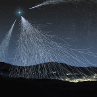
Cherenkov Radiation
It may sound like the name of a ames Bond villain, but this phenomenon is actually our maximum object of study
Cherenkov radiation is the electromagnetic radiation emitted when a charged particle passes through a dielectric medium at a speed greater than the phase velocity of light in that medium. When a very energetic gamma photon or cosmic ray interacts with the Earth’s atmosphere, a high-speed cascade of particles is produced. The Cherenkov radiation of these charged particles is used to determine the origin and intensity of cosmic or gamma rays.
Find out more:

Cherenkov Telescopes
Our favourite toys!
Cherenkov telescopes are high-energy gamma photon detectors located on the Earth’s surface. They have a mirror to gather light and focus it towards the camera. They detect light produced by the Cherenkov effect from blue to ultraviolet on the electromagnetic spectrum. The images taken by the camera allow us to identify if the particular particle in the atmosphere is a gamma ray and at the same time determine its direction and energy. The MAGIC telescopes at Roque de Los Muchachos (La Palma) are an example.
Find out more:

Cosmic Rays
You need to know how to distinguish between rays, particles and sparks!
Cosmic rays are examples of high-energy radiation composed mainly of highly energetic protons and atomic nuclei. They travel almost at the speed of light and when they hit the Earth’s atmosphere, they produce cascades of particles. These particles generate Cherenkov radiation and some can even reach the surface of the Earth. However, when cosmic rays reach the Earth, it is impossible to know their origin, because their trajectory has changed. This is due to the fact that they have travelled through magnetic fields which force them to change their initial direction.
Find out more:
Dark Matter
What can it be?
How can we define something that is unknown? We know of its existence because we detect it indirectly thanks to the gravitational effects it causes in visible matter, but we can’t study it directly. This is because it doesn’t interact with the electromagnetic force so we don’t know what it is composed of. Here, we are talking about something that represents 25% of everything known! So, it’s better not to discount it, but rather try to shed light on what it is …
Find out more:

Duality Particle Wave
But, what is it?
A duality particle wave is a quantum phenomenon in which particles take on the characteristics of a wave, and vice versa, on certain occasions. Things that we would expect to always act like a wave (for example, light) sometimes behave like a particle. This concept was introduced by Louis-Victor de Broglie and has been experimentally demonstrated.
Find out more:

Event
These really are the events of the year
When we talk about events in this field, we refer to each of the detections we make via telescopes. For each of them, we have information such as the position in the sky, the intensity, and so on. This information allows us to classify them. We are interested in having many events so that we can carry out statistical analysis a posteriori and draw conclusions.

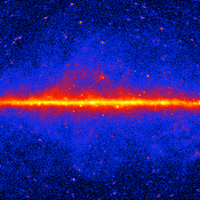
Gamma Ray
Yes, we can!
Gamma rays are extreme-frequency electromagnetic ionizing radiation (above 10 exahertz). They are the most energetic range on the electromagnetic spectrum. The direction from which they reach the Earth indicates where they originate from.
Find out more:
Lorentz Covariance
The privileges of certain equations.
Certain physical equations have this property, by which they don’t change shape when certain coordinates changes are given. The special theory of relativity requires that the laws of physics take the same form in any inertial reference system. That is, if we have two observers whose coordinates can be related by a Lorentz transformation, any equation with covariant magnitudes will be written the same in both cases.
Find out more:

Microquasar
Below you will learn what a quasar is...well a microquasar is the same, but smaller!
A microquasar is a binary star system that produces high-energy electromagnetic radiation. Its characteristics are similar to those of quasars, but on a smaller scale. Microquasars produce strong and variable radio emissions often in the form of jets and have an accretion disk surrounding a compact object (e.g. a black hole or neutron star) that’s very bright in the range of X-rays.
Find out more:

Nebula
What shape do the clouds have?
Nebulae are regions of the interstellar medium composed basically of gases and some chemical elements in the form of cosmic dust. Many stars are born within them due to condensation and accumulation of matter. Sometimes, it’s just the remains of extinct stars.
Find out more:

Particle Shower
The Niagara Falls of particles!
A particle shower results from the interaction between high-energy particles and a dense medium, for example, the Earth’s atmosphere. In turn, each of these secondary particles produced creates a cascade of its own, so that they end up producing a large number of low-energy particles.

Pulsar
Now you see me, now you don't
The word ‘pulsar’ comes from the shortening of pulsating star and it is precisely this, a star from which we get a discontinuous signal. More formally speaking, it’s a neutron star that emits electromagnetic radiation while it’s spinning. The emissions are due to the strong magnetic field they have and the pulse is related to the rotation period of the object and the orientation relative to the Earth. One of the best known and studied is the pulsar of the Crab Nebula, which, by the way, is very beautiful.
Find out more:

Quantum Gravity
A union of 'grave' importance ...
This field of physics aims to unite the quantum field theory, which applies the principles of quantum mechanics to classical systems of continuous fields, and general relativity. We want to define a unified mathematical basis with which all the forces of nature can be described, the Unified Field Theory.
Find out more:

Quasar
A 'quasi' star
Quasars are the furthest and most energetic members of a class of objects called active core galaxies. The name, quasar, comes from ‘quasi-stellar’ or ‘almost stars’. This is because, when they were discovered, using optical instruments, it was very difficult to distinguish them from the stars. However, their emission spectrum was clearly unique. They have usually been formed by the collision of galaxies whose central black holes have merged to form a supermassive black hole or a binary system of black holes.
Find out more:

Supernova Remnant
A candy floss in the cosmos
When a star explodes (supernova) a nebula structure is created around it, formed by the material ejected from the explosion along with interstellar material.
Find out more:

Theory of relativity
In this life, everything is relative...or not!
Albert Einstein was the genius who, with his theories of special and general realtivity, took Newtonian mechanics and made it compatible with electromagnetism. The first theory is applicable to the movement of bodies in the absence of gravitational forces and in the second theory, Newtonian gravity is replaced with more complex formulas. However, for weak fields and small velocities it coincides numerically with classical theory.
Find out more:
